Figures on this page are conceptual illustrations built from synthetic geometry. They are not customer layouts, captured files, or measured benchmarks. The card image is a supplied illustration of layered geometry and parallel execution; its layer names and left-to-right CPU strip are visual labels, not a process stack or a claim that machines run in sequence.
Generating a useful synthetic workload is a systems problem. A small set of rules has to produce large, structured geometry; that geometry has to be stored without copying what never changes; and the work has to be split so independent slices can run at the same time. The interesting question is how those three choices interact.
The Challenge: Scale Changes Everything
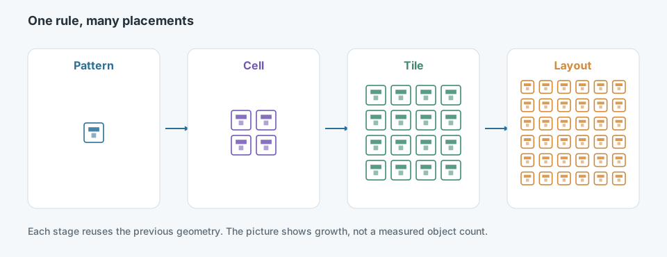
The same rule is applied again at each stage. The drawing shows the idea of growth. It does not report how many objects a real workload contains.
A few thousand objects can be drawn, stored, and checked directly. At a much larger scale, the same approach changes the problem:
- Volume. Object count, spatial extent, and the number of output files all grow together.
- Memory. Materializing every copy of a repeated shape keeps data that a reference could have named.
- Computation. Placement, validation, and export repeat work that does not depend on neighboring slices.
- Repetition. Structured fields contain the same cell many times. The repetition is the opportunity and the storage risk.
- Reproducibility. A later run has to recover the same geometry from the same configuration, including any controlled variation.
- Partitioning. A workload that cannot be cut into independent slices cannot be retried or distributed without redoing everything.
The implemented framework is configurable across geometric patterns, spatial distributions, tile settings, and workload scale. It generates synthetic data so evaluation does not depend on customer layouts.
Rule-Based Geometric Synthesis
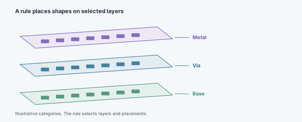
Layer names in this figure are illustrative categories. They are not a description of a specific manufacturing stack.
The generator starts from configuration rather than from a drawing of every object. The documented controls cover geometric pattern rules, spatial distribution, tile configuration, and workload scale. A useful configuration answers a few concrete questions:
- How large is one tile, and how are tiles arranged?
- Which geometric patterns are allowed, and where may they be placed?
- Which layers participate, and which spatial constraints keep objects from colliding or drifting?
- Which variations are intentional, and which values must stay fixed so a run can be repeated?
Those choices are the product. Once they are explicit, the same configuration can describe a small test field or a much larger one without redrawing the geometry.
Efficient Geometric Representation
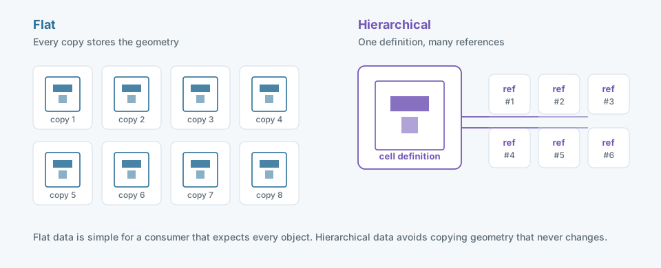
Flat data repeats the geometry. Hierarchical data names a reusable cell and records where each instance goes.
A flat representation writes every object explicitly. Any consumer can read it without resolving references, and random access is straightforward. The cost is duplication: a cell that appears throughout a field is stored throughout the field.
A hierarchical representation stores the cell once and records instances by reference and transformation. Storage and memory follow the number of distinct definitions more closely than the number of placements. The cost moves to the reader, which must resolve references, and to any downstream tool that only accepts flat geometry.
The implemented system uses hierarchical geometry reuse for layout storage. In one documented comparison of a representative swath, the hierarchical layout file was about 3 KB where the flat file was about 530 KB, a 99.4% reduction in that file. That number describes one file-size comparison. It is not a measurement of runtime, memory during generation, or cluster throughput.
Generation and export do not have to use the same representation. A pipeline can build geometry from reusable cells and still flatten the result when a consumer cannot follow references. The storage win and the compatibility requirement are separate decisions.
Pipeline Architecture
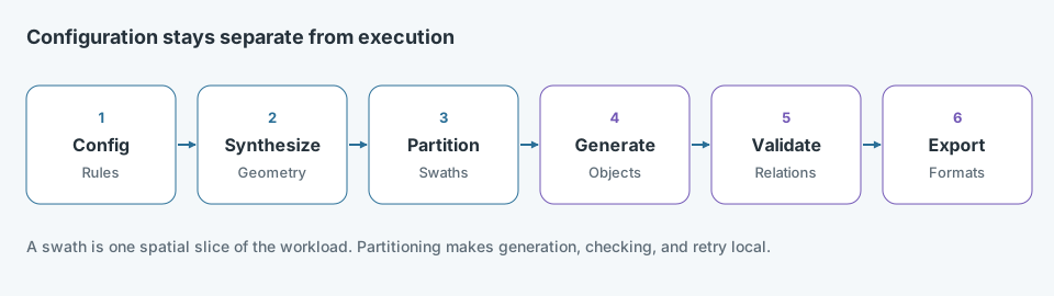
Partitioning comes before the expensive generation so each slice can be produced, checked, and retried on its own.
The documented pipeline keeps several outputs in agreement: generated layout geometry, structured configuration or recipe data, spatial metadata, and registration locations. They share a coordinate system and explicit relationships, so a coordinate in one output still refers to the same place in the others.
The engineering choices behind that flow are ordinary and important:
- Cut the workload into swaths. A swath is one spatial slice. It is the unit of generation, not a machine and not a processing stage.
- Keep configuration outside the execution loop. Changing scale or pattern rules should not require rewriting the worker.
- Avoid carrying unused intermediates. A slice should produce the outputs that later stages actually read.
- Record enough to repeat the run. The configuration, seed, and slice identity are part of the result, not an afterthought.
The diagram is a conceptual ordering of those responsibilities. It is not an internal architecture drawing.
Parallel Execution & Scalability
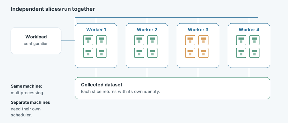
Each worker receives a different slice at the same time. The pool collects results after those slices finish.
The implemented execution model partitions the workload by swath and runs those slices with configurable CPU multiprocessing. Independent slices do not need each other’s geometry, so they can proceed together and be collected afterward.
That is different from scheduling the same work across separate machines. Multiprocessing shares one machine’s CPUs, memory, and disks. A multi-machine run adds placement, network transfer, and failure handling that this page does not claim were built for this generator. High-performance computing appears in related layout-processing work; it is not described here as the scheduler for synthetic workload generation.
More workers are not automatically more throughput. The useful limits are:
- Granularity. A very small slice adds scheduling and file overhead. A very large slice reduces the chance to balance work and retry a failure.
- Concurrency. Extra processes compete for the same memory and the same disks.
- I/O. Writing many layout and metadata files can dominate once geometry generation is no longer the slow part.
- Balance. Slices with different pattern density finish at different times. The pool waits on the slow slice unless the partition accounts for that.
- Isolation. A failed slice should be rerun from its configuration. It should not require regenerating the whole field.
Data Outputs & Validation
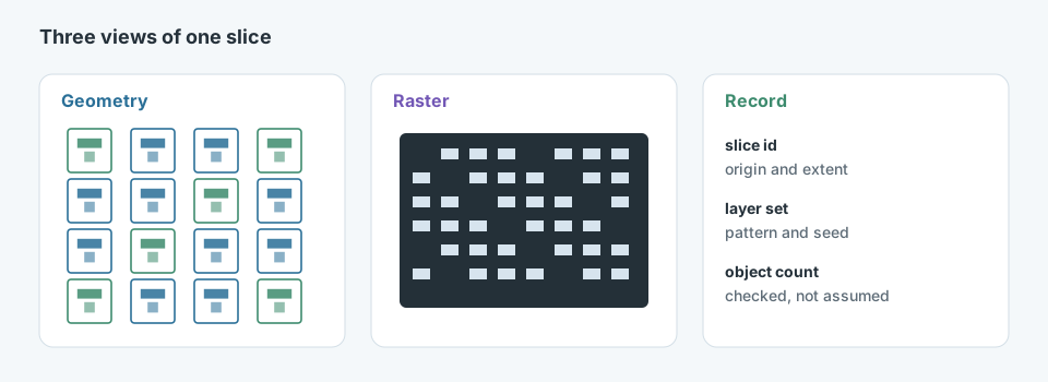
The record fields are examples of the kind of information a slice needs. They are not a captured metadata file.
A generated workload is usable when its outputs describe the same structure. The documented set includes layout geometry, structured recipe or configuration data, spatial metadata, and registration locations. Raster views and coordinate lists are natural companions when a consumer needs pixels or explicit positions; this page does not treat every possible export as a verified format.
Validation checks the relationships, not only that files exist. A registration location should fall inside the slice it names. A metadata extent should match the geometry. A repeated run with the same configuration should land on the same objects. Metadata is what makes that check possible after the geometry has left the generator.
Engineering Challenges & Trade-offs
Flat vs. hierarchical
Hierarchical reuse avoids storing unchanged cells again, which is why the representative swath file became much smaller. Flat export remains appropriate when a downstream reader cannot resolve references. The representation used internally and the representation written for a consumer can differ.
Task granularity
Swath partitioning makes retries and multiprocessing possible. Cutting finer adds scheduling and file overhead; cutting coarser leaves less room to balance dense and sparse regions. The slice size is a workload decision, not a constant.
Parallelism vs. contention
Configurable multiprocessing uses CPUs that would otherwise sit idle. Past the point where workers contend for memory or disk, adding a process increases occupancy without increasing completed slices. The bottleneck has to be identified before the worker count is treated as a speed setting.
Flexibility vs. reproducibility
Pattern, distribution, tile, and scale controls make one framework serve many evaluations. They also make accidental change easy. A run is reproducible only when the configuration, controlled variation, and slice identity are stored with the outputs.
Results & Engineering Insights
What was built
A configurable generator for synthetic geometric workloads, with pattern, distribution, tile, and scale controls, and without dependence on customer layouts.
What was measured
One representative comparison: hierarchical reuse reduced a per-swath layout file from about 530 KB to about 3 KB. No end-to-end throughput or cluster-scaling result is reported here.
What the design supports
The framework is designed to support billion-scale synthetic datasets for inspection, registration, and scalability evaluation. “Designed to support” is a capacity goal, not a completed benchmark.
What has to stay consistent
Layout, configuration data, spatial metadata, and registration locations are useful together only when they share coordinates and can be checked against one another.
Scale shows up where representation, computation, and I/O meet. Hierarchical storage removes repeated geometry from the file. Swath partitioning removes repeated work from the critical path. Multiprocessing uses that independence, until memory and disk become the limit. A configuration that can be stored and rerun is what keeps those optimizations from turning a large dataset into an unreproducible one.